Understanding the Magnetic Field Around a Current-Carrying Wire: B = μ₀I/2πr Explained

Have you ever wondered how the magnetic field around a current-carrying wire is formed? The intriguing formula, B = μ₀I/2πr — The Magnetic Field Around a Current-Carrying Wire, offers a fascinating glimpse into this phenomenon. Whether you’re a student, a physics enthusiast, or simply curious, understanding this concept is crucial in unraveling the mysteries of electromagnetism. As we delve into this topic, we’ll explore how a simple electrical current can create a magnetic field, affecting everything from household appliances to complex industrial machinery.

To truly grasp the significance of this formula and its applications, it’s essential to start with the basics of electromagnetism. According to Ampère’s Circuital Law, the magnetic field generated around a wire is directly proportional to the current flowing through it and inversely proportional to the distance from the wire. This means that as the current increases or as you move closer to the wire, the magnetic field’s strength also increases.

Understanding these principles not only enriches your knowledge of physics but also highlights the beauty and complexity of the natural world. For more insights into the fascinating world of electromagnetism, visit our home page where we delve into more exciting topics.

Introduction to Magnetic Fields and Current-Carrying Wires

Magnetic fields are an intrinsic part of the universe, influencing various aspects of our daily lives and technological advancements. The interaction between electricity and magnetism is a cornerstone of electromagnetism, a field that has revolutionized our understanding of natural forces. When a wire carries an electrical current, it creates a magnetic field around it. This phenomenon is not only central to modern physics but also to numerous practical applications, from household devices to advanced scientific instruments.

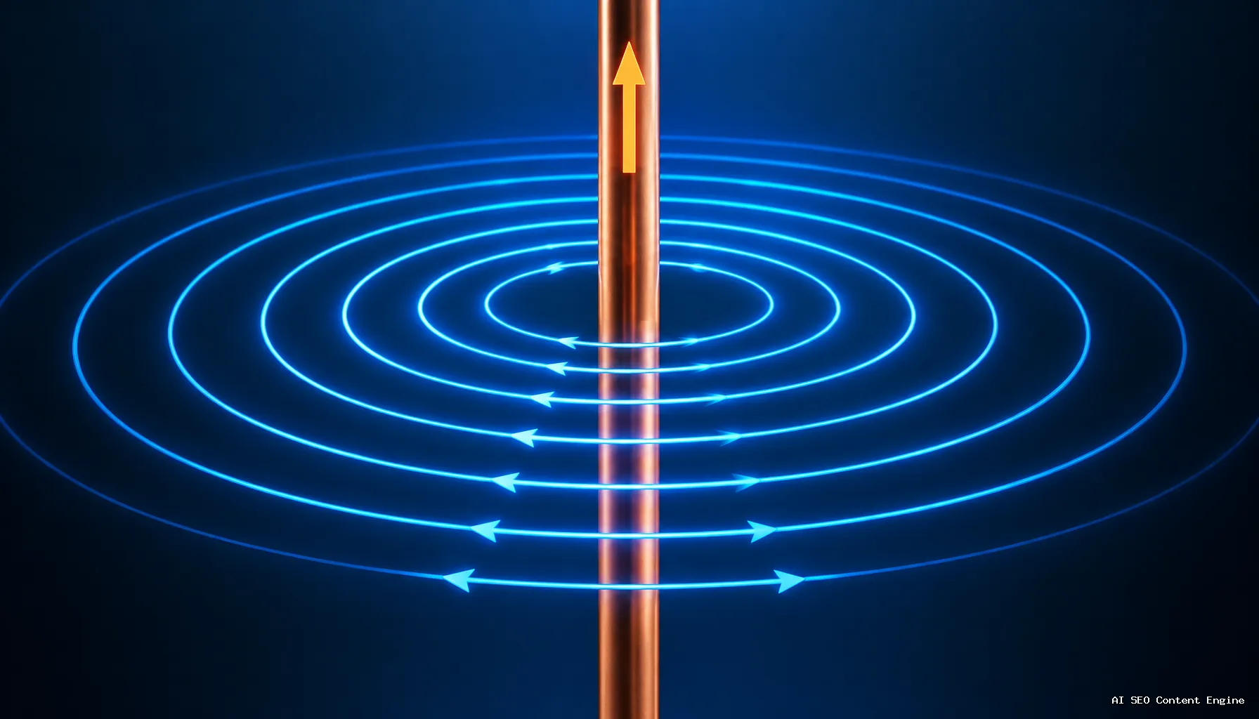
The concept of magnetic fields around current-carrying wires was first discovered by Hans Christian Ørsted in the early 19th century. Ørsted’s discovery revealed that an electric current produces a circular magnetic field, which can be visualized using the right-hand rule. This simple yet powerful tool allows us to determine the direction of the magnetic field relative to the direction of current flow: if you point your thumb in the direction of the current, your fingers curl in the direction of the magnetic field.

Understanding the Basics

To comprehend how magnetic fields are generated by electrical currents, it’s crucial to explore some foundational concepts:

• Biot-Savart Law: This law provides a mathematical framework to calculate the magnetic field produced by a small segment of current-carrying wire. It helps in understanding how the field strength varies with distance and current.
• Ampère’s Law: A pivotal principle that relates the magnetic field in a closed loop to the electric current passing through the loop. It offers a broader understanding of magnetic field calculations, especially for symmetrical configurations like solenoids and toroids.

These principles lay the groundwork for exploring more intricate phenomena, such as the magnetic fields inside solenoids, which are coils of wire that intensify the magnetic field when current passes through them.

Moreover, as we delve deeper into the mechanics of electromagnetism, we find applications of these principles in various domains. For example, understanding how magnetic fields interact with buoyant forces can enhance our grasp of concepts like Archimedes’ Principle and Its Role in Buoyancy, expanding our appreciation for the interconnected nature of physical laws.

By mastering these concepts, not only do we gain insight into the behavior of magnetic fields around current-carrying wires, but we also unlock a deeper understanding of the natural and technological world. This knowledge is invaluable for anyone interested in physics, engineering, or simply the marvels of electromagnetism.

The Formula B = μ₀I/2πr: Breaking Down the Components

The formula B = μ₀I/2πr provides a fundamental way to calculate the magnetic field around a straight, current-carrying wire. Understanding each component of this equation is crucial for grasping how magnetic fields operate in relation to electric currents.

Understanding the Components

• B (Magnetic Field): This represents the magnetic field intensity at a point located at a distance r from the wire. It is measured in Tesla (T).
• μ₀ (Permeability of Free Space): This constant signifies the extent to which a magnetic field can penetrate space. Its value is approximately 4π x 10^-7 T·m/A. It is a crucial factor in magnetic field calculations.
• I (Current): The electric current flowing through the wire, measured in Amperes (A). The direction of this current is essential for applying the right-hand rule to determine the direction of the magnetic field.
• r (Distance): The perpendicular distance from the wire to the point where the magnetic field is being calculated. The magnetic field decreases with increasing distance from the wire, illustrating an inverse relationship.

Physical Interpretation and Application

This equation stems from the Biot-Savart law, which describes the magnetic field generated by a current element. It is particularly useful for calculating fields in symmetric situations, such as around long straight wires. The right-hand rule can be applied here to determine the direction of the magnetic field: if you point your thumb in the direction of the current, your fingers will curl in the direction of the magnetic field lines.

The derivation and application of this formula are rooted in historical discoveries, notably Ørsted’s observation that electric currents affect compass needles, thereby linking electricity and magnetism. For more complex configurations, such as solenoids or loops, Ampere’s law and the Biot-Savart law offer additional insights.

Understanding this formula is not only crucial for academic purposes but also has practical implications in engineering and technology. For instance, it helps in designing electromagnets and understanding how magnetic fields interact with other forces.

By breaking down and understanding the components of this formula, we gain a deeper appreciation of the principles governing the interaction between electricity and magnetism, highlighting the elegance and interconnectedness of physical laws.

Historical Insights: From Ørsted to Modern Applications

The journey of understanding the magnetic field around a current-carrying wire begins with a pivotal moment in the early 19th century when Hans Christian Ørsted first observed that electric currents could deflect a magnetic compass needle. This groundbreaking discovery in 1820 provided the first clear evidence of a relationship between electricity and magnetism, setting the stage for the development of electromagnetic theory.

Ørsted’s Discovery

Ørsted’s experiments demonstrated that a magnetic field is produced around a wire carrying an electric current. This phenomenon was a major turning point in the study of physics, as it introduced the concept that electricity and magnetism were intrinsically linked. Ørsted’s findings led to further research by scientists such as André-Marie Ampère, who formulated Ampere’s law, describing the magnetic field generated by an electric current in a more mathematical form.

Developments in Electromagnetic Theory

• Ampere’s Law: This law quantifies the relationship between an electric current and the magnetic field it produces. It allows us to calculate the magnetic field strength in various configurations, particularly useful for understanding solenoids and other complex systems.
• Biot-Savart Law: Complementing Ampere’s law, the Biot-Savart law provides a method to determine the magnetic field at a point in space due to a small segment of current-carrying conductor. It is essential for calculating fields in cases where the symmetry required by Ampere’s law is absent.

Modern Applications

Today, the principles outlined by Ørsted, Ampère, and others have been instrumental in the development of numerous technologies. The ability to calculate and predict magnetic fields is crucial in the design and operation of electrical devices such as transformers, electric motors, and generators. These applications demonstrate the enduring significance of early scientific discoveries in modern engineering and technology.

Furthermore, understanding the interaction of magnetic fields with other forces is vital in fields like medical imaging (MRI) and telecommunications. For instance, when designing systems that rely on magnetic fields, engineers must consider the effects of these fields on surrounding materials and devices, including potential influences on buoyancy as described in Archimedes’ Principle and Its Role in Buoyancy.

In summary, the historical insights from Ørsted’s observations have paved the way for a deeper understanding of electromagnetic interactions, enabling significant advancements in both theoretical physics and practical applications. The exploration of these principles continues to inspire innovation and discovery in the ever-evolving field of electromagnetism.

The Right-Hand Rule: Determining Magnetic Field Direction

After delving into the profound implications of Ørsted’s discovery and the mathematical elegance of the Biot-Savart Law, it is crucial to understand the practical methods used to determine the direction of the magnetic field generated by a current-carrying wire. This is where the right-hand rule becomes an indispensable tool for physicists and engineers alike.

Understanding the Right-Hand Rule

The right-hand rule provides a simple yet powerful way to visualize the orientation of the magnetic field around a wire. To apply the right-hand rule:

• Point your right thumb in the direction of the current flow through the wire.
• Curl your fingers around the wire. The direction in which your fingers naturally curl represents the circular path of the magnetic field lines around the wire.

This intuitive method effectively illustrates how the magnetic fields surround current-carrying conductors, facilitating easier magnetic field calculations and predictions of electromagnetic interactions.

Applications and Importance

The right-hand rule is not only applicable to straight wires but also extends to more complex configurations such as solenoids and loops. In these cases, the rule helps in determining the orientation of the magnetic field lines within and around these structures, which is essential for designing electromagnetic devices and understanding their behavior.

Moreover, applying this rule aids engineers in predicting how magnetic fields will interact with other systems, which is crucial in fields like telecommunications and medical imaging. For instance, when designing MRI machines, understanding the magnetic field orientation ensures accurate imaging and safety.

Further Exploration

For those interested in exploring related principles, such as how buoyancy can be influenced by magnetic fields, consider reading our article on Archimedes’ Principle and Its Role in Buoyancy. Such interdisciplinary insights reveal the interconnected nature of physical laws and their applications.

In summary, the right-hand rule is a fundamental concept that enhances our ability to visualize and predict the behavior of magnetic fields in various scenarios. Its simplicity and effectiveness make it an enduring tool in the study and application of electromagnetism.

Factors Influencing Magnetic Field Strength

Understanding the factors that affect the strength of a magnetic field around a current-carrying wire is crucial for both theoretical and practical applications. Several key elements contribute to the intensity and behavior of the magnetic field generated by electrical currents.

Current Intensity

The strength of the magnetic field is directly proportional to the current flowing through the wire. A higher current results in a stronger magnetic field. This relationship is fundamental to electromagnetic applications, where altering current levels can modulate the magnetic field strength to suit specific needs.

Distance from the Wire

The distance from the wire is inversely proportional to the magnetic field strength. As you move further away from the wire, the magnetic field weakens. This is a critical consideration in magnetic field calculations, especially when determining the field’s influence on nearby objects or systems.

Permeability of the Medium

The medium surrounding the wire also plays a role in the magnetic field’s strength. The magnetic permeability of the material reflects its ability to support the formation of a magnetic field. Materials with higher permeability, such as iron, can enhance the magnetic field, while non-magnetic materials have little effect.

Wire Configuration

The configuration of the wire influences the magnetic field as well. A straight wire produces a different magnetic field pattern compared to coiled configurations like solenoids, which can intensify the magnetic field within the coil. This principle is utilized in the design of electromagnets and other electromagnetic devices.

By understanding these factors, engineers and scientists can better predict and manipulate magnetic fields in various applications, from telecommunications to medical imaging.

Comparing Magnetic and Electric Field Decay

Understanding the decay of fields, both magnetic and electric, is vital in comprehending how forces act over distance. While both fields originate from charges, their behavior as they extend outward shows distinct characteristics.

Decay Patterns

The magnetic field around a current-carrying wire, as described by the equation B = μ₀I/2πr, diminishes with distance from the wire. This inverse relationship means that the magnetic field strength decreases as one moves further away, following a 1/r decay pattern. This is critical for applications where proximity to the magnetic source is a factor, such as in designing circuits and understanding how solenoids operate.

In contrast, electric fields produced by point charges decay according to an inverse square law, represented by the formula F = kq₁q₂/r². This indicates that the electric field strength drops more rapidly with distance than the magnetic field, a distinction that impacts how these fields are utilized in different technologies.

Influencing Factors

• Source Configuration: Just as a coiled wire can alter the magnetic field, configurations such as parallel plates influence electric fields, demonstrating the importance of design in field manipulation.
• Application of Ørsted’s Discovery: The realization that an electric current affects a magnetic compass needle laid the groundwork for understanding how magnetic fields decay, offering insights into practical applications like the right-hand rule for determining field direction.
• Role of Ampere’s Law and Biot-Savart Law: These laws further describe how current and distance affect magnetic fields, providing tools for precise magnetic field calculation and enhancing our grasp of field interactions.

Ultimately, the difference in decay rates between magnetic and electric fields influences how they are applied in real-world scenarios. While electrical forces are crucial for applications requiring rapid diminishment, magnetic fields are preferred where a longer-range influence is desirable.

Applications of Magnetic Fields in Everyday Life

Magnetic fields are fundamental to a wide range of applications that impact our daily lives, from the technology we use to the medical procedures that ensure our health and safety. By understanding how magnetic fields behave, such as those around a current-carrying wire, we can harness their properties for innovative solutions and improvements.

Technology and Electronics

One of the most prevalent uses of magnetic fields is in the realm of electronics. Devices like hard drives and speakers rely on magnetic fields to function. Hard drives use magnetic fields to read and write data, a process crucial for data storage and retrieval. Similarly, speakers convert electrical energy into mechanical energy using magnets to produce sound.

Medical Applications

Magnetic fields play a vital role in the medical field, particularly in imaging and diagnostic tools. Magnetic Resonance Imaging (MRI) exploits strong magnetic fields to generate detailed images of the inside of the human body, aiding in the diagnosis of various medical conditions. The non-invasive nature of MRI makes it an indispensable tool in modern medicine.

Transportation and Navigation

Magnetic fields are also critical in transportation systems. Magnetic levitation (maglev) trains utilize magnetic fields for propulsion and levitation, reducing friction and allowing for high-speed travel. Additionally, navigation systems have long depended on the Earth’s magnetic field; compasses, an ancient tool, continue to be essential for directional guidance.

Industrial and Power Generation

In industries, magnetic fields are used in various processes, including the separation of materials and the operation of electric motors and generators. These motors and generators convert electrical energy to mechanical energy and vice versa, forming the backbone of modern power generation and distribution systems.

Overall, the versatile nature of magnetic fields, governed by principles such as Ørsted’s discovery and the Biot-Savart Law, ensures their continued relevance and utility in advancing technology and enhancing quality of life.

Conclusion

In summary, the formula B = μ₀I/2πr offers a fundamental understanding of the magnetic field produced by a current-carrying wire. By appreciating the relationship between the current, the permeability of free space, and the distance from the wire, we gain insights into the behavior of magnetic fields in practical applications. This knowledge is essential not only for academic purposes but also for its applications in electrical engineering and technology development. As we continue to explore the complexities of electromagnetism, this foundational principle remains a cornerstone in understanding the interactions between electricity and magnetism.

Frequently Asked Questions

What happens when a current-carrying wire is kept in a magnetic field?

When a current-carrying wire is placed in a magnetic field, it experiences a force perpendicular to both the direction of the current and the magnetic field. This phenomenon is described by the Lorentz force law, which states that the force on the wire is given by F = I(L × B), where F is the force, I is the current, L is the length of the wire in the magnetic field, and B is the magnetic field. This principle is utilized in devices such as electric motors and generators.

What is the magnetic field strength at a distance of 2 cm from a wire carrying a current of 5 A?

Using the formula B = μ₀I/2πr, where μ₀ (the permeability of free space) is approximately 4π × 10⁻⁷ T·m/A, I is the current, and r is the distance from the wire, we can calculate the magnetic field strength. At a distance of 2 cm (0.02 m) from a wire carrying a current of 5 A, the magnetic field strength is approximately B = (4π × 10⁻⁷ T·m/A × 5 A) / (2π × 0.02 m) = 5 × 10⁻⁵ T or 50 μT.

Why is Ampere’s law used for the derivation in magnetic field due to a long straight current-carrying wire of infinite length and not Biot Savart’s law?

Ampere’s law is often used for deriving the magnetic field around a long straight current-carrying wire of infinite length because it simplifies the calculation by taking advantage of the symmetry of the problem. Ampere’s law relates the integrated magnetic field around a closed loop to the current passing through the loop, making it particularly efficient for problems with high symmetry such as an infinite wire. In contrast, Biot-Savart’s law, while more general, is more complex for such symmetric configurations as it involves integrating over the length of the wire.

What is Biot-Savart law class 12 simple derivation?

The Biot-Savart law provides a mathematical model to calculate the magnetic field produced by a small segment of current-carrying wire. For a small segment dl of a wire carrying current I, the magnetic field dB at a point in space is given by dB = (μ₀/4π) * (I dl × r̂) / r², where r is the distance from the segment to the point of interest and r̂ is the unit vector from the segment to the point. To derive the total magnetic field, one would integrate this expression over the entire current distribution. This law is fundamental in understanding the magnetic effects of currents in arbitrary-shaped conductors.