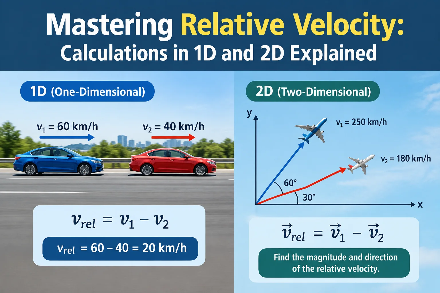
Mastering Relative Velocity: Calculations in 1D and 2D Explained

Have you ever watched two cars speeding down a highway and wondered how fast they are moving relative to each other? Understanding how to calculate relative velocity in 1D and 2D is crucial for anyone diving deep into the world of physics or engineering. Whether you’re a student tackling your first physics problem or a professional brushing up on essentials, mastering this concept can help you visualize and solve real-world motion problems with precision.

In this comprehensive guide, we’ll unravel the mysteries of relative velocity, providing you with clear explanations and step-by-step calculations in both one-dimensional and two-dimensional spaces. Prepare to transform your understanding of motion and gain the confidence to tackle complex problems with ease.

Understanding Relative Velocity

Relative velocity is a fundamental concept in physics that describes the motion of an object as observed from another moving object. It is an essential component of kinematics, specifically when dealing with problems involving multiple moving objects, such as cars on a highway or planes in the sky. Understanding relative velocity helps in analyzing and solving problems related to motion, whether in one dimension (1D) or two dimensions (2D).

What is Relative Velocity?

In simple terms, relative velocity is the velocity of an object as observed from another moving object. It provides a way to compare the motion of two objects in relation to each other. The concept is vital in both one-dimensional (1D) and two-dimensional (2D) motion analysis.

Relative Velocity Formula

The relative velocity of object A with respect to object B is given by:

V_AB = V_A – V_B

Where:

• V_AB is the relative velocity of object A with respect to object B.
• V_A is the velocity of object A.
• V_B is the velocity of object B.

This simple formula applies to both 1D and 2D scenarios, where the velocities are considered vectors.

Relative Motion in 1D

In one-dimensional motion, objects move along a straight line. Understanding relative velocity in 1D involves considering the direction and speed of each object. For example, if two cars are moving along a straight road, the relative velocity can help determine how fast they are approaching or receding from each other.

**Solved Example:** If Car A is moving at 60 km/h and Car B is moving at 40 km/h in the same direction, the relative velocity of Car A with respect to Car B is:

V_AB = 60 km/h – 40 km/h = 20 km/h

Relative Motion in 2D

When objects move in a plane, their motion is described in two dimensions, involving both horizontal and vertical components. In 2D kinematics, relative velocity calculations become more complex, as they require vector addition and subtraction.

**Example Scenario:** Consider two birds flying in the sky. Bird A is flying north at 10 m/s, and Bird B is flying east at 5 m/s. To find the relative velocity of Bird A with respect to Bird B, you would use vector addition to combine these motions.

**Solution:**

• Bird A’s velocity vector: (0, 10) m/s
• Bird B’s velocity vector: (5, 0) m/s
• Relative velocity: V_AB = (0 – 5, 10 – 0) = (-5, 10) m/s

Understanding these concepts is crucial for solving more complex problems involving relative motion in 2D, such as determining the trajectory of an aircraft relative to wind or the movement of a boat in a river current.

As you delve deeper into relative velocity, practice solving problems by applying these principles and using the relative velocity formula. This will enhance your ability to visualize and calculate motion in both simple and complex scenarios.

Relative Velocity in One Dimension

Calculating relative velocity in one dimension is a fundamental concept in physics, providing a foundation for understanding motion in more complex scenarios. In this section, we will explore the principles behind relative velocity in a linear path, also known as 1D motion. This type of motion is simpler to analyze compared to relative motion in 2D, as it involves only scalar quantities rather than vectors.

Understanding Relative Velocity in 1D

Relative velocity refers to the velocity of one object as observed from another moving object. In one-dimensional motion, this calculation involves straightforward arithmetic due to the linear nature of the path. The basic idea is to find out how fast one object is moving in relation to another.

Relative Velocity Formula

The formula for calculating relative velocity in one dimension is:

V_AB = V_A – V_B

• V_AB: Relative velocity of object A with respect to object B.
• V_A: Velocity of object A.
• V_B: Velocity of object B.

In this formula, both velocities (V_A and V_B) are considered in the same direction along a straight line. The subtraction accounts for the relative differences in their speeds.

Solved Problems on Relative Motion in 1D

Let’s look at a few examples to solidify the concept:

Example 1:

Consider two cars traveling along a straight road. Car A is moving at 60 km/h, while Car B is moving in the same direction at 40 km/h. What is the relative velocity of Car A with respect to Car B?

Solution:

• V_A = 60 km/h
• V_B = 40 km/h
• V_AB = V_A – V_B = 60 km/h – 40 km/h = 20 km/h

The relative velocity of Car A with respect to Car B is 20 km/h.

Example 2:

Suppose Car A is moving at 80 km/h east, and Car B is moving at 50 km/h west. What is the relative velocity of Car A with respect to Car B?

Solution:

• V_A = 80 km/h (east)
• V_B = -50 km/h (west direction is considered negative in this context)
• V_AB = V_A – V_B = 80 km/h – (-50 km/h) = 130 km/h

The relative velocity of Car A with respect to Car B is 130 km/h, indicating how fast Car A is moving away from Car B.

Understanding these basic calculations in one dimension is essential before tackling more complex problems involving relative motion in 2D. Practice with various scenarios will enhance your problem-solving skills and prepare you for advanced kinematics challenges.

Applying the Relative Velocity Formula in 1D

The concept of relative velocity in one dimension (1D) is foundational for understanding motion in physics. It allows us to determine how fast one object is moving relative to another when both are moving along a straight line. This understanding sets the stage for more complex analyses in 2D kinematics and relative motion in 2D.

Understanding the Formula

The relative velocity formula in 1D is straightforward: the relative velocity of object A with respect to object B (denoted as V_AB) is calculated by subtracting the velocity of object B (V_B) from the velocity of object A (V_A). Mathematically, it is expressed as:

V_AB = V_A – V_B

This formula is particularly useful in solving problems where two objects are moving along the same line, either towards each other or in the same direction. The sign of the velocities plays a crucial role, as it indicates the direction of motion.

Key Considerations in 1D Relative Velocity

• Direction Matters: In 1D problems, direction is indicated by the sign of the velocity. For example, if two cars are moving in opposite directions, one velocity might be positive while the other is negative.
• Frame of Reference: Always establish a frame of reference before solving a problem. Decide which direction is positive and which is negative to avoid confusion.
• Same Direction: When two objects move in the same direction, the relative velocity is the difference in their speeds.
• Opposite Direction: When objects move towards each other, the relative velocity is effectively the sum of their speeds due to the subtraction of a negative velocity.

Practical Application

Applying the relative velocity formula in 1D involves recognizing the direction and speed of the objects involved. Here’s a step-by-step approach:

1. Identify the velocities of both objects and their directions.
2. Assign positive or negative signs to velocities based on their direction in your chosen frame of reference.
3. Use the relative velocity formula: V_AB = V_A – V_B.
4. Interpret the result: A positive relative velocity indicates that object A is moving away from object B, while a negative value suggests it is moving towards object B.

Practicing with solved problems on relative motion will enhance your understanding and ability to approach more complex problems involving relative velocity in one dimension problems and answers. Mastery of these concepts is essential as you progress towards analyzing relative motion in 2D scenarios.

Example Problems and Solutions for 1D

Understanding relative velocity in one dimension can be solidified through practical examples. In this section, we will explore a few example problems that illustrate how to calculate relative velocity in 1D. These solved problems on relative motion will help clarify the concept and improve your problem-solving skills.

Problem 1: Cars on a Highway

Imagine two cars, Car A and Car B, traveling on a straight highway. Car A is moving at a velocity of 60 km/h east, while Car B is moving at 40 km/h east.

• Step 1: Assign directions and magnitudes:
  
  – Velocity of Car A, \( V_A = +60 \, \text{km/h} \)
  
  – Velocity of Car B, \( V_B = +40 \, \text{km/h} \)
  
• Step 2: Use the relative velocity formula:
  
  – \( V_{AB} = V_A – V_B \)
  
  – \( V_{AB} = 60 \, \text{km/h} – 40 \, \text{km/h} = 20 \, \text{km/h} \)
  
• Step 3: Interpretation:
  
  – The positive relative velocity indicates Car A is moving away from Car B at 20 km/h.
  

Problem 2: Train Passing a Stationary Observer

A train travels at 80 km/h towards the east while an observer stands stationary on the platform.

• Step 1: Directions and magnitudes:
  
  – Velocity of the train, \( V_T = +80 \, \text{km/h} \)
  
  – Velocity of the observer, \( V_O = 0 \, \text{km/h} \)
  
• Step 2: Calculate relative velocity:
  
  – \( V_{TO} = V_T – V_O \)
  
  – \( V_{TO} = 80 \, \text{km/h} – 0 \, \text{km/h} = 80 \, \text{km/h} \)
  
• Step 3: Interpretation:
  
  – The train appears to move past the observer at 80 km/h.
  

Problem 3: Opposite Directions

Consider two joggers on a track. Jogger A runs at 10 km/h east, while Jogger B runs at 8 km/h west.

• Step 1: Assign signs based on direction:
  
  – Velocity of Jogger A, \( V_A = +10 \, \text{km/h} \)
  
  – Velocity of Jogger B, \( V_B = -8 \, \text{km/h} \)
  
• Step 2: Apply the relative velocity formula:
  
  – \( V_{AB} = V_A – V_B \)
  
  – \( V_{AB} = 10 \, \text{km/h} – (-8) \, \text{km/h} = 18 \, \text{km/h} \)
  
• Step 3: Interpretation:
  
  – Jogger A is moving away from Jogger B at 18 km/h, accounting for their opposite directions.
  

Practicing these examples will deepen your comprehension of relative velocity in one dimension, paving the way to tackle more challenging problems in 2D kinematics and relative motion in 2d.

Relative Velocity in Two Dimensions

Transitioning from understanding relative velocity in one-dimensional motion, we now delve into the more complex realm of two-dimensional motion, where vectors play a crucial role. This extends our comprehension beyond linear paths to include movements in planes, such as those encountered in real-world scenarios like aviation, sailing, and meteorology.

Understanding the Concept

Relative velocity in two dimensions involves the calculation of velocity vectors along both the x and y axes. This requires breaking down the motion into components and using vector addition or subtraction to find the relative velocity. Consider the following:

• Vector Components: Each object’s velocity is expressed as a vector with horizontal (x) and vertical (y) components.
• Vector Addition: The relative velocity is determined by adding or subtracting these components from each other.

Relative Velocity Formula in 2D

To calculate relative velocity in two dimensions, use the following formula:

\[ \overrightarrow{V_{AB}} = \overrightarrow{V_A} – \overrightarrow{V_B} \]

Where:

• \(\overrightarrow{V_A}\) and \(\overrightarrow{V_B}\) are the velocity vectors of objects A and B, respectively.
• Each vector is expressed as \((V_{Ax}, V_{Ay})\) and \((V_{Bx}, V_{By})\), representing the x and y components.

Example Problem: Solving Relative Motion in 2D

Consider two airplanes, Plane C and Plane D. Plane C flies with a velocity of \(400 \, \text{km/h}\) at a \(30^\circ\) angle north of east, while Plane D flies at \(380 \, \text{km/h}\) due east.

Step 1: Break Down Into Components

• Plane C:
  • \(V_{Cx} = 400 \cdot \cos(30^\circ) = 346.41 \, \text{km/h}\)
  • \(V_{Cy} = 400 \cdot \sin(30^\circ) = 200 \, \text{km/h}\)
• Plane D:
  • \(V_{Dx} = 380 \, \text{km/h}\)
  • \(V_{Dy} = 0 \, \text{km/h}\)

Step 2: Calculate the Relative Velocity

• \(V_{CDx} = V_{Cx} – V_{Dx} = 346.41 – 380 = -33.59 \, \text{km/h}\)
• \(V_{CDy} = V_{Cy} – V_{Dy} = 200 – 0 = 200 \, \text{km/h}\)

The relative velocity vector \(\overrightarrow{V_{CD}}\) is \((-33.59, 200) \, \text{km/h}\).

Step 3: Interpretation

The negative x-component indicates Plane C is moving slower eastward compared to Plane D, while the positive y-component shows Plane C is moving northward relative to Plane D. The magnitude of the relative velocity can be calculated using the Pythagorean theorem:

\[ |\overrightarrow{V_{CD}}| = \sqrt{(-33.59)^2 + (200)^2} = 202.80 \, \text{km/h} \]

This example illustrates how breaking velocities into components and applying vector mathematics can solve complex problems in 2D kinematics. By practicing such solved problems on relative motion, one gains deeper insights into the dynamics of systems moving in two dimensions.

Vector Components and Equations of Motion

Understanding vector components and equations of motion is crucial for calculating relative velocity, especially in two-dimensional (2D) scenarios. This section will delve into the intricacies of vectors and how they are applied in relative motion in 2D, providing a solid foundation for tackling solved problems on relative motion.

Breaking Down Vectors into Components

Vectors, by nature, have both magnitude and direction. To effectively analyze motion, especially in a plane, vectors are often broken down into components. In two dimensions, any vector can be represented by its x-component and y-component. This decomposition is essential for using the relative velocity formula effectively.

• X-Component: Represents the horizontal influence of a vector. Calculated as \(V_x = V \cdot \cos(\theta)\), where \(V\) is the vector’s magnitude and \(\theta\) is the angle with the horizontal axis.
• Y-Component: Represents the vertical influence of a vector. Calculated as \(V_y = V \cdot \sin(\theta)\).

By breaking vectors into these components, we simplify complex motions into manageable calculations.

Equations of Motion in 1D and 2D

The equations of motion are mathematical expressions that describe the behavior of a moving object. In the context of relative velocity, these equations help to determine how an object’s position changes over time relative to another object.

1D Equations of Motion

In one-dimensional motion, the equations are straightforward:

• \(v = u + at\), where \(v\) is the final velocity, \(u\) is the initial velocity, \(a\) is the acceleration, and \(t\) is the time.
• \(s = ut + \frac{1}{2}at^2\), where \(s\) is the displacement.
• \(v^2 = u^2 + 2as\).

These equations are crucial when analyzing relative velocity in one dimension problems and answers.

2D Kinematics

For two-dimensional motion, the situation becomes more complex but follows similar principles:

• Vector Addition: Combine x and y components using vector addition to find resultant vectors.
• Relative Motion in 2D: Use component-wise addition or subtraction to find relative velocities.
• Application of Trigonometry: Often necessary to resolve vectors and find angles.

In practice, calculating relative velocity in 2D involves breaking down each object’s velocity into components, applying the relative velocity formula component-wise, and then recomposing the results into a single vector.

By mastering these vector components and equations of motion, one can solve complex problems in 2D kinematics with ease, leading to a deep understanding of dynamics in motion systems. This knowledge is indispensable for students and professionals working with relative motion scenarios.

Solving Relative Velocity Problems in 2D

Solving relative velocity problems in two dimensions requires a systematic approach that involves breaking down vectors into their components, applying vector addition rules, and occasionally using trigonometric functions to resolve the vectors. Here’s how you can tackle these problems effectively:

Step-by-Step Approach

1. 
   Identify the Objects and Their Velocities: Begin by clearly identifying the objects involved in the problem and their respective velocities. These velocities should be considered as vectors, having both magnitude and direction.
   
2. Break Down the Vectors into Components: Each velocity vector should be decomposed into its x and y components. This is typically done using:
   • The formulas: \( V_x = V \cdot \cos(\theta) \) and \( V_y = V \cdot \sin(\theta) \), where \( V \) is the magnitude of the velocity and \( \theta \) is the angle.
   • Employing these transformations allows for straightforward addition or subtraction of velocities in each dimension separately.
3. Apply the Relative Velocity Formula: The relative velocity \( \mathbf{V}_{AB} \) of object A with respect to object B can be determined by:
   • Subtracting the velocity vector of B from A: \( \mathbf{V}_{AB} = \mathbf{V}_A – \mathbf{V}_B \).
   • Perform this calculation component-wise for both x and y directions:
     • \( V_{AB_x} = V_{A_x} – V_{B_x} \)
     • \( V_{AB_y} = V_{A_y} – V_{B_y} \)
4. Recompose the Resultant Vector: Once the components of the relative velocity are found, they can be recombined to form the resultant vector. Utilize the Pythagorean theorem:
   
   
   
   • \( V_{AB} = \sqrt{(V_{AB_x})^2 + (V_{AB_y})^2} \)
   
   
   
   

   This gives the magnitude of the relative velocity.

   
   
5. Determine the Direction: The direction of the relative velocity can be found using trigonometry:
   
   
   
   • \( \theta = \tan^{-1}\left(\frac{V_{AB_y}}{V_{AB_x}}\right) \)
   
   
   
   

   This angle is typically measured from the positive x-axis.

   
   

Practical Application

To solidify understanding, practice with solved problems on relative motion is essential. For instance, determining the relative velocity of a boat crossing a river while accounting for water current involves applying these principles, where understanding the interplay of velocities helps predict the boat’s actual path.

Incorporating these methods not only enhances problem-solving skills but also deepens comprehension of physical systems, making it easier to tackle complex dynamics scenarios found in various fields of physics and engineering.

Practical Applications and Common Mistakes

Understanding relative velocity in both one-dimensional (1D) and two-dimensional (2D) contexts is crucial for solving real-world problems in physics and engineering. Whether it’s analyzing the motion of vehicles on a highway or determining the trajectory of an aircraft relative to the wind, these concepts are widely applicable. Here, we delve into some practical applications and highlight common mistakes that can lead to errors in calculations.

Practical Applications

1. Navigation and Transportation

In navigation, especially maritime and aviation, calculating relative motion in 2D is essential. For instance, when a pilot charts a course, they must account for wind speed and direction to maintain a desired flight path. This is a direct application of the relative velocity formula:

• **Aircraft Navigation**: Pilots use relative velocity to ensure they reach their destination efficiently. They calculate the relative velocity concerning air currents to adjust their heading and speed.
• **Maritime Transport**: Captains calculate the relative velocity of their ships concerning ocean currents to determine the most efficient route.

2. Sports and Ballistics

In sports, understanding relative motion helps in strategies and performance improvement:

• **Ball Sports**: In games like baseball or cricket, players consider the relative velocity of the ball concerning their own motion to predict its trajectory and make successful plays.
• **Ballistics**: Military applications often involve calculating the relative velocity of projectiles concerning targets, accounting for factors like wind and target movement.

Common Mistakes

Despite its broad applicability, several common mistakes can occur when calculating relative velocity:

Misinterpretation of Reference Frames

One of the most frequent errors is choosing the wrong reference frame. It’s critical to clearly define which object is stationary and which is moving relative to that object. For example:

• When solving relative velocity in one dimension problems and answers, ensure you have a consistent point of reference throughout the problem.

Ignoring Direction

Especially in 2D kinematics, neglecting the direction can lead to incorrect conclusions:

• **Vector Components**: Always break down velocities into their vector components and apply the correct trigonometric functions to solve for magnitude and direction.
• **Sign Convention**: Be consistent with the sign convention (positive or negative) when dealing with opposite directions.

Incorrect Application of Formulas

Errors often arise from the misuse of formulas:

• **Relative Velocity Formula**: Ensure you apply the formula \( V_{AB} = V_A – V_B \) correctly, considering the direction of each velocity vector.
• **Complex Problems**: When dealing with solved problems on relative motion, carefully follow each step of the solution to understand the application of principles.

By being mindful of these practical applications and common pitfalls, you can enhance your problem-solving skills in relative velocity, making it easier to tackle complex dynamics scenarios found in various fields of physics and engineering.

Frequently Asked Questions

What is Relative Velocity?

Relative velocity refers to the velocity of one object as observed from another moving object. It is a crucial concept in understanding how different observers perceive motion differently depending on their own motion. This concept is widely used in physics to analyze scenarios where multiple objects are in motion, such as cars on a highway or aircraft in flight.

How Do You Calculate Relative Velocity in One Dimension?

In one-dimensional motion, the relative velocity formula is straightforward:

• Formula: \( V_{AB} = V_A – V_B \)

Here, \( V_{AB} \) is the relative velocity of object A with respect to object B. The calculation involves simple subtraction of the velocities, keeping in mind the direction as indicated by the sign convention.

How is Relative Velocity Calculated in Two Dimensions?

Calculating relative velocity in two dimensions (2D kinematics) involves vector addition and subtraction. Each velocity is broken down into its components:

• X-component: \( V_{ABx} = V_{Ax} – V_{Bx} \)
• Y-component: \( V_{ABy} = V_{Ay} – V_{By} \)

To find the magnitude of the relative velocity, use the Pythagorean theorem:

• Magnitude: \( V_{AB} = \sqrt{(V_{ABx})^2 + (V_{ABy})^2} \)

This approach is essential in relative motion in 2D, especially when dealing with problems involving vectors at angles.

Can You Provide an Example Problem?

Let’s consider a solved problem on relative motion:

Example: Two cars are moving along a straight highway. Car A is moving at 60 km/h, and Car B at 40 km/h in the same direction. What is the relative velocity of Car A with respect to Car B?

• Solution: Using the formula \( V_{AB} = V_A – V_B \), we find \( V_{AB} = 60 \text{ km/h} – 40 \text{ km/h} = 20 \text{ km/h} \).

This means Car A is moving at 20 km/h relative to Car B.

What Are Common Mistakes in Solving Relative Velocity Problems?

Common errors include:

• Ignoring Direction: Misinterpreting the direction can lead to incorrect results. Always pay attention to the sign (positive or negative) of velocity components.
• Misapplying Formulas: Ensure correct application of the relative velocity formula, considering vector directions for 2D problems.

By understanding these common mistakes, you can improve your ability to solve relative velocity in one dimension problems and answers effectively.

Why is Understanding Relative Velocity Important?

Understanding relative velocity is crucial in fields such as physics and engineering, where analyzing motions relative to different reference frames is necessary. It helps in solving complex problems involving multiple moving objects, enhancing your problem-solving skills in dynamics and kinematics.

Conclusion

Understanding how to calculate relative velocity in both one-dimensional and two-dimensional spaces is crucial for solving various physics problems. By grasping the concept of relative velocity, you can better analyze situations involving multiple moving objects, such as vehicles on a road or celestial bodies in space. Whether you are a student or a professional, mastering these calculations enhances your analytical skills and deepens your comprehension of motion dynamics. As you continue to explore the principles of relative velocity, you will find it easier to apply these concepts to real-world scenarios, making complex motion analysis more intuitive and accessible.