Vectors and Scalars: Definitions, Examples, and How to Master Vector Addition

Introduction to Vectors and Scalars: Understanding the Basics

Understanding the fundamental concepts of vectors and scalars is critical for diving into physics, engineering, and various fields of mathematics. At their core, they represent different types of quantities. Scalars are quantities that are described by a magnitude alone. Think about temperature, mass, or distance. For instance, saying “the temperature is 30 degrees Celsius” gives a clear, complete picture without needing any additional information.

On the other hand, vectors deal with quantities that require both magnitude and direction. Velocity and force are prime examples. When you say, “the car is moving at 60 kilometers per hour to the north,” you provide not just the speed but also the direction of motion. This distinction is crucial because it influences how we solve problems related to motion and forces.

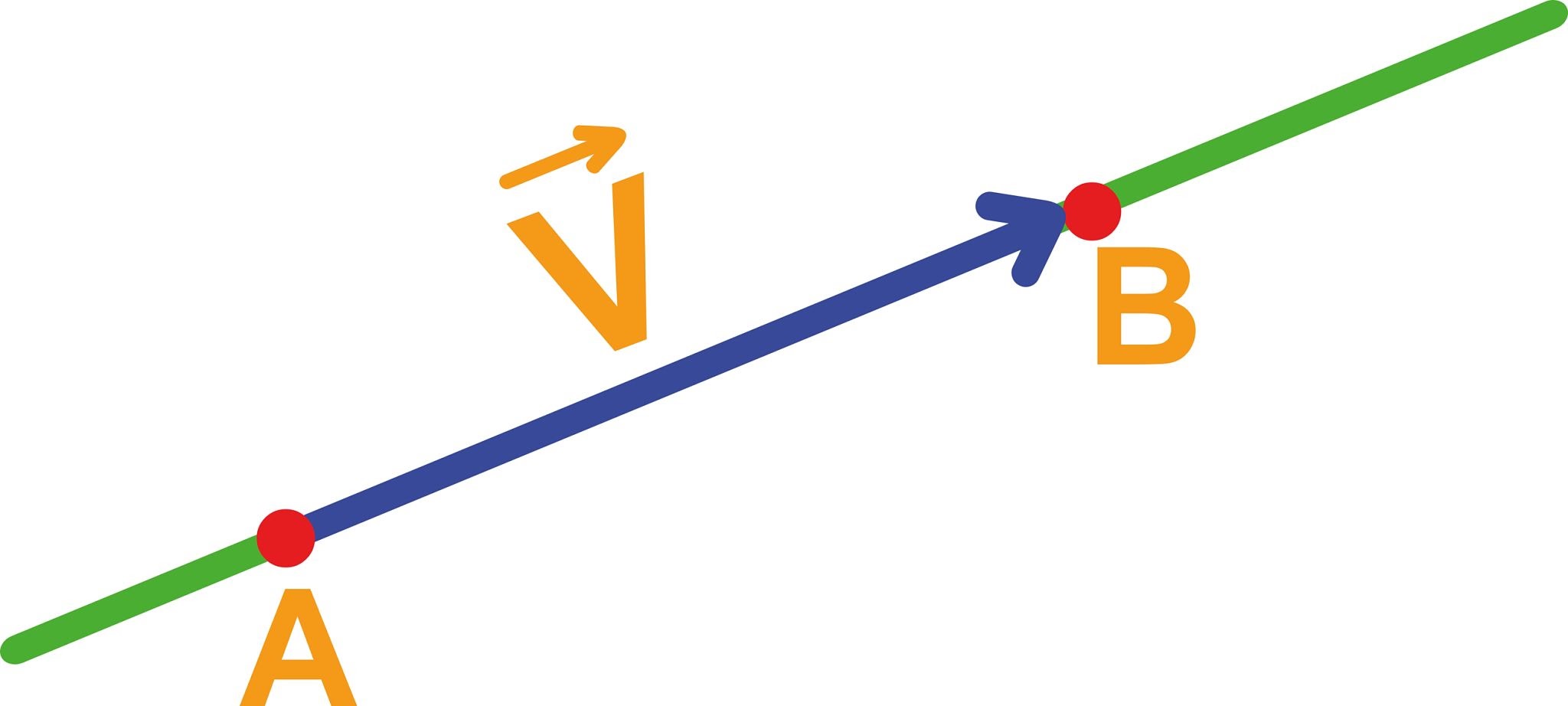
Visualizing these concepts can be incredibly helpful. Scalars can be represented simply as points on a number line. You can easily see their magnitude but there’s no direction associated. Vectors, however, are often depicted as arrows in a coordinate system. The length of the arrow indicates the magnitude, while the arrowhead points in the direction of the vector.

Another key aspect is how these quantities interact. Scalars can be added or subtracted straightforwardly. For example, if you have two distances, 5 meters and 3 meters, adding them gives you a clear result: 8 meters. Vectors, however, require a more nuanced approach due to their directional component. Adding two vectors involves not just summing their lengths but also considering their angles relative to one another. This process can be visualized using graphical methods or calculated using trigonometry.

In practical applications, the distinction between vectors and scalars often dictates the approach you’ll take in problem-solving. For instance, in physics simulations, recognizing whether a quantity is a vector or a scalar can change how you calculate interactions. Scalars can often be manipulated with basic arithmetic, while vector operations might involve more complex rules like the parallelogram law or the triangle method.

Grasping these differences lays the groundwork for mastering vector addition and other advanced topics. As you proceed, keep these foundational concepts in mind; they will serve as stepping stones for more complex ideas and calculations.

Defining Scalars: Characteristics and Examples

Scalars are fundamental quantities in physics and mathematics that possess only magnitude, devoid of any direction. This simplicity is what sets them apart from vectors, which incorporate both magnitude and direction. Understanding scalars is crucial, as they form the building blocks for more complex concepts in physics and engineering.

One of the primary characteristics of scalars is that they can be described with a single numerical value. For instance, temperature, mass, and speed are all scalars. When you say the temperature is 30 degrees Celsius, you provide a specific magnitude without indicating any direction. This characteristic makes scalars easier to work with in many mathematical operations.

Let’s explore some common examples of scalars:

• Temperature: Measured in degrees Celsius or Fahrenheit, temperature indicates how hot or cold an object is. It is a scalar because it does not require a directional component; 20°C is simply 20°C, regardless of where you are.
• Mass: This is the amount of matter in an object, typically measured in kilograms or grams. Whether an object weighs 5 kg or 10 kg, there’s no direction involved—it’s purely a measure of quantity.
• Speed: Unlike velocity, which includes direction, speed represents how fast an object is moving. For example, if a car travels at 60 kilometers per hour, it’s moving at a rate that doesn’t specify the direction of travel.
• Energy: Energy can be quantified as potential energy, kinetic energy, and thermal energy. Whether it’s 50 joules of kinetic energy or 200 joules of potential energy, the value alone provides the necessary information about the energy present.
• Time: Measured in seconds, minutes, or hours, time is another scalar quantity. Saying an event lasts for 30 minutes gives a clear magnitude without any directional context.

Scalars can also be manipulated using basic arithmetic operations. You can add, subtract, multiply, or divide scalars easily. For example, if you have a mass of 5 kg and you add another 3 kg, you simply get 8 kg. There’s no need to consider direction, making calculations straightforward.

In contrast, when dealing with vectors, you must pay attention to both magnitude and direction. This distinction highlights the utility of scalars in various fields, including physics, engineering, and everyday applications. Scalars allow for simplicity in calculations, making them indispensable in scientific and mathematical contexts.

Understanding scalars not only enhances your grasp of physical concepts but also lays the groundwork for mastering more complex topics like vectors and their operations. Recognizing how scalars function in isolation helps clarify their role in vector addition and other advanced mathematical operations.

Defining Vectors: Key Properties and Examples

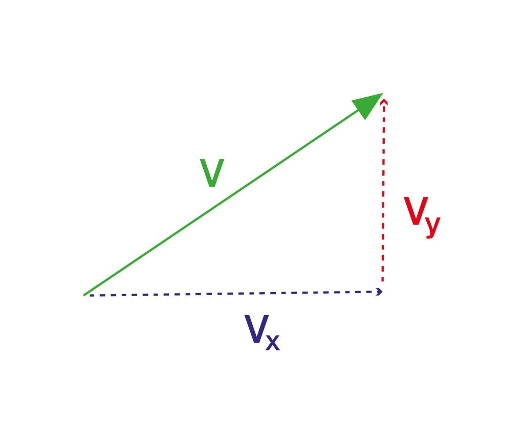
Vectors are fundamental entities in mathematics and physics, characterized by both magnitude and direction. To fully grasp vectors, understanding their key properties is crucial. These properties distinguish vectors from scalars, which only have magnitude.

First, let’s talk about **magnitude**. This is simply the length or size of a vector. In mathematical terms, if we have a vector represented as \(\mathbf{v} = (x, y)\), the magnitude can be calculated using the formula:

\[ ||\mathbf{v}|| = \sqrt{x^2 + y^2} \]

Consider a vector \(\mathbf{v} = (3, 4)\). The magnitude is:

\[ ||\mathbf{v}|| = \sqrt{3^2 + 4^2} = \sqrt{9 + 16} = \sqrt{25} = 5 \]

Next comes **direction**. This is how a vector points in space. It’s often expressed as an angle relative to a reference axis. For instance, if the angle of \(\mathbf{v}\) with respect to the positive x-axis is \(θ\), then you can determine the direction using trigonometric functions:

\[ \tan(θ) = \frac{y}{x} \]

Using the previous example, for \(\mathbf{v} = (3, 4)\):

\[ \tan(θ) = \frac{4}{3} \]

Calculating this gives \(θ ≈ 53.13°\). Thus, the vector points in a specific direction in a 2D plane.

**Vector addition** is another critical concept. When adding two vectors, the resultant vector is obtained by placing the tail of one vector at the head of the other. This can be visually represented using the triangle or parallelogram method. For example, if vector \(\mathbf{u} = (1, 2)\) and vector \(\mathbf{v} = (3, 4)\), their sum \(\mathbf{u} + \mathbf{v} = (1+3, 2+4) = (4, 6)\).

Let’s not forget about **unit vectors**. A unit vector has a magnitude of 1 and points in the direction of the original vector. To convert a vector to a unit vector, divide it by its magnitude. For instance, the unit vector of \(\mathbf{v} = (3, 4)\) is:

\[ \hat{\mathbf{v}} = \frac{\mathbf{v}}{||\mathbf{v}||} = \left(\frac{3}{5}, \frac{4}{5}\right) \]

This shows how the direction remains intact while normalizing the length to 1.

Finally, vectors can be expressed in different **coordinate systems**. For example, in Cartesian coordinates, we use \( (x, y) \) pairs, while in polar coordinates, we express vectors using magnitude and angle \( (r, θ) \). This flexibility allows for various applications depending on the context, such as physics, engineering, or computer graphics.

Understanding these properties and examples of vectors lays the groundwork for mastering more complex concepts, like vector operations and applications in real-world scenarios.

The Importance of Vectors and Scalars in Physics and Mathematics

Understanding vectors and scalars is fundamental in both physics and mathematics, influencing how we interpret and interact with the world around us. Vectors and scalars serve distinct but interconnected roles that help us describe motion, forces, and various physical phenomena.

Scalars are quantities that have magnitude only. For example, temperature, mass, and speed are scalars. You can say it’s 30 degrees Celsius, the mass is 5 kilograms, or the speed is 60 kilometers per hour. Each of these examples provides a clear value but lacks direction. Scalars are crucial in various calculations, especially in thermodynamics and statistics, where only the size of the quantity matters.

In contrast, vectors possess both magnitude and direction. Velocity is a prime example. You can say a car is moving at 60 kilometers per hour to the north. This description gives both the speed and the direction of the car’s travel. Vectors are essential in physics, particularly in mechanics, where they are used to represent forces, velocity, acceleration, and displacement. Without vectors, we wouldn’t be able to capture the full behavior of dynamic systems.

Both vectors and scalars are vital in mathematical formulations. In fields like calculus and linear algebra, vectors can be manipulated through addition, subtraction, and multiplication. Understanding these operations is essential for solving complex problems that involve multiple dimensions, such as in computer graphics or engineering simulations.

Additionally, the interplay between vectors and scalars provides deeper insights into physical laws. Newton’s laws of motion, for instance, incorporate forces (vectors) acting on objects with mass (a scalar). This relationship helps us predict how objects will move under various influences.

In summary, mastering the concepts of vectors and scalars enhances our ability to describe and analyze the physical world. Whether you’re calculating forces in a physics problem or analyzing data in a mathematical context, recognizing the differences and applications of these quantities is crucial. Grasping these concepts not only aids in academic pursuits but also lays the groundwork for practical applications in engineering, computer science, and many other fields.

Vector Notation and Representation: Graphical and Algebraic Methods

Understanding how to represent vectors is fundamental to mastering vector addition. Vectors can be expressed in two primary ways: graphically and algebraically. Each method offers unique advantages and helps in visualizing and solving problems in physics and engineering.

Graphical Representation of Vectors

Graphical representation involves drawing vectors on a coordinate system, typically a two-dimensional plane. Each vector is represented as an arrow. The direction of the arrow indicates the vector’s direction, while its length corresponds to its magnitude.

To draw a vector, you start at a point, known as the tail, and extend the arrow to another point, called the head. For example, if you have a vector \( \mathbf{A} \) that has a magnitude of 5 units and points 30 degrees above the horizontal axis, you can draw it using a protractor for accuracy.

It’s useful to note that vectors can be added graphically using the head-to-tail method. To add two vectors, place the tail of the second vector at the head of the first. The resultant vector is drawn from the tail of the first vector to the head of the second. This visual method makes it easier to grasp vector addition intuitively.

Algebraic Representation of Vectors

Algebraically, vectors are expressed using components. In a two-dimensional Cartesian coordinate system, a vector \( \mathbf{A} \) can be represented as \( \mathbf{A} = (A_x, A_y) \), where \( A_x \) and \( A_y \) are the components of the vector along the x-axis and y-axis, respectively.

To convert from a magnitude and angle to components, you can use trigonometric functions. For a vector with magnitude \( A \) and angle \( \theta \), the components are given by:

– \( A_x = A \cdot \cos(\theta) \)
– \( A_y = A \cdot \sin(\theta) \)

For instance, if you have a vector \( \mathbf{B} \) with a magnitude of 10 units at an angle of 45 degrees, the components become:

– \( B_x = 10 \cdot \cos(45^\circ) = 7.07 \)
– \( B_y = 10 \cdot \sin(45^\circ) = 7.07 \)

Thus, \( \mathbf{B} = (7.07, 7.07) \).

Combining Graphical and Algebraic Methods

Often, it’s beneficial to use both methods together. You can draw the vectors graphically to visualize their direction and magnitude, then use the algebraic representations to perform calculations. This combination is powerful in solving complex problems involving multiple vectors.

Understanding how to switch between these representations enhances your ability to tackle vector addition problems effectively. With practice, you’ll find that recognizing the relationships between the graphical and algebraic forms becomes second nature, paving the way for mastering vector operations.

Understanding Vector Addition: The Triangle and Parallelogram Laws

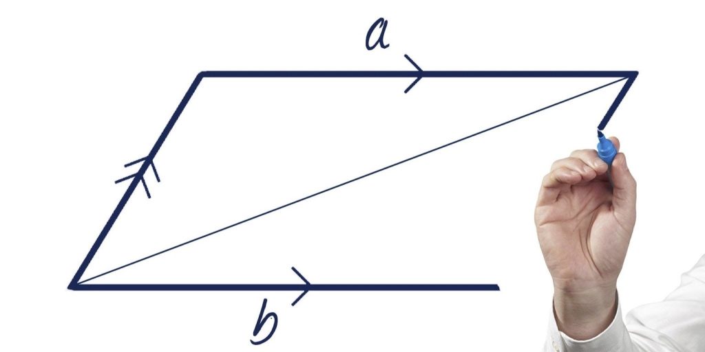
Vector addition is essential in physics and engineering, and two main methods help visualize and compute it: the triangle law and the parallelogram law. Mastering these concepts can enhance your grasp of vector operations and their applications.

The triangle law of vector addition is relatively straightforward. Imagine you have two vectors, A and B. To add them, place the tail of vector B at the head of vector A. The resultant vector, R, is drawn from the tail of vector A to the head of vector B. This method visually illustrates how vectors combine directionally. For example, if vector A points east with a magnitude of 5 units and vector B points north with a magnitude of 3 units, the resultant vector R can be found by constructing a right triangle. This triangle’s sides represent the original vectors, and R is the hypotenuse.

Next, let’s dive into the parallelogram law. This method is particularly useful when adding two vectors that are not perpendicular. To apply the parallelogram law, you still start with vectors A and B. Draw both vectors from a common origin, then complete a parallelogram by drawing lines parallel to each vector. The diagonal of this parallelogram represents the resultant vector R. This method is especially handy when dealing with vectors that are at angles to each other, allowing you to determine the magnitude and direction of the resultant vector with ease.

Mathematically, the triangle law can be expressed as R = A + B, while the parallelogram law can be represented using the formula R² = A² + B² + 2AB cos(θ), where θ is the angle between vectors A and B. This formula enables you to calculate the magnitude of the resultant vector when you know the magnitudes of the original vectors and the angle between them.

In practice, understanding these laws allows for more effective problem-solving in physics. Whether you’re calculating forces acting on an object or determining velocities in motion, these addition methods are foundational. By mastering them, you’ll not only improve your analytical skills but also gain confidence in tackling more complex vector problems.

Common Mistakes in Vector Addition and How to Avoid Them

Ignoring Directions

One of the most frequent mistakes when adding vectors is neglecting their directions. Vectors are not just about magnitude; their direction is crucial. For instance, if you have a vector pointing east and another pointing west, you can’t simply add their magnitudes. You need to account for their directions.

To avoid this mistake, always visualize or draw the vectors. Use a coordinate system to place them accurately. This method not only helps in understanding their relative positions but also clarifies how they interact. When vectors oppose each other, remember to subtract the smaller magnitude from the larger one, keeping the direction of the resultant vector in mind.

Failing to Use the Correct Units

Mixing units is a common pitfall. If one vector is measured in meters and another in kilometers, you’ll end up with an incorrect resultant vector. Consistency in units is vital for accurate vector addition.

To sidestep this error, always convert your measurements to the same unit before performing any calculations. This ensures that your final answer will be coherent and logical. A simple conversion factor can save you from significant mistakes down the line.

Incorrectly Applying the Triangle Method

The triangle method is a popular way to visualize vector addition, but it’s often misapplied. It’s crucial to arrange the vectors head-to-tail accurately. If you misalign them, the resultant vector will be off.

To avoid this, take your time when drawing. Start with the first vector, then attach the second vector to the head of the first. The line from the tail of the first vector to the head of the second gives you the resultant vector. Double-check your angles to ensure they reflect the correct directions.

Neglecting the Pythagorean Theorem for Perpendicular Vectors

When adding vectors that are perpendicular, many forget to apply the Pythagorean theorem correctly. If two vectors are at right angles, the magnitude of the resultant vector is not just the sum of their lengths.

Instead, you must square both magnitudes, add those squares, and then take the square root to find the resultant. To sidestep this, remember the formula:

\[
R = \sqrt{A^2 + B^2}
\]

where \(R\) is the resultant vector, and \(A\) and \(B\) are the magnitudes of the two vectors.

Conclusion

Awareness of these common mistakes is the first step towards mastering vector addition. By paying attention to directions, maintaining unit consistency, accurately applying the triangle method, and correctly using the Pythagorean theorem, you can enhance your skills and avoid pitfalls in vector addition. With practice, these principles will become second nature, leading to a deeper understanding of vectors and their applications.

Practical Applications of Vectors and Scalars in Real-Life Scenarios

Vectors and scalars are more than just theoretical concepts; they play a crucial role in various real-world applications. Let’s break down how each is used across different fields to illustrate their significance.

Vectors in Navigation

Take navigation, for instance. When pilots or sailors chart a course, they rely heavily on vectors. The direction and speed of the aircraft or vessel are represented as vectors. For example, if a plane is flying north at 500 miles per hour, that’s a vector. If it encounters a wind blowing east at 100 miles per hour, the resultant vector—determining its actual path—can be calculated using vector addition. This ensures that they reach their destination efficiently, despite external factors.

Scalars in Everyday Measurements

Scalars are found in everyday measurements, such as temperature and distance. When you say it’s 30 degrees Celsius outside, that’s a scalar measurement. It gives you a precise value without any direction involved. Similarly, if you drive 50 miles to work, that distance is a scalar. It tells you how far you traveled but not the direction you took.

Vectors in Physics and Engineering

In physics, vectors are fundamental. Consider forces acting on an object. If you push a box with a force of 10 newtons to the east and another person pushes it with 5 newtons to the north, the net force acting on the box is a vector sum of these forces. Understanding this helps engineers design structures that can withstand varying forces, ensuring safety in construction.

Scalars in Financial Analysis

In finance, scalars are used for analyzing profits and expenses. When a business reports a profit of $200,000, that’s a scalar. It provides a straightforward figure that helps stakeholders assess financial health without considering direction. This scalar information is vital for making informed investment decisions.

Vectors in Sports

Sports also utilize vectors extensively. In soccer, the speed and angle at which a player kicks the ball can be represented as vectors. This data can be analyzed to improve player performance. Coaches often use vector analysis to strategize plays, ensuring players know their positioning relative to the goal and each other.

Understanding vectors and scalars allows us to interpret the world more effectively. Whether navigating the skies, measuring temperature, calculating forces, or making financial decisions, these concepts are at the heart of countless applications. The next time you encounter these terms, remember their real-life implications. They are not just numbers; they are tools that shape our understanding and actions in various domains.

Exercises to Master Vector Addition: Step-by-Step Problems

Understanding the Basics

Before diving into exercises, let’s quickly review what vector addition entails. You add vectors by combining their magnitudes and directions. Vectors can be represented graphically as arrows, where the length indicates magnitude and the direction shows orientation.

Exercise 1: Basic Vector Addition

Consider two vectors: **A** = 3 units to the right and **B** = 4 units upwards. To find the resultant vector **R**, you can use the graphical method.

1. **Draw Vector A**: Start at the origin and draw a horizontal arrow 3 units long to the right.
2. **Draw Vector B**: From the head of Vector A, draw a vertical arrow 4 units long upwards.
3. **Resultant Vector R**: Draw a diagonal line from the tail of Vector A to the head of Vector B. Use the Pythagorean theorem to find the magnitude of **R**.

\[ R = \sqrt{(3^2 + 4^2)} = \sqrt{25} = 5 \text{ units} \]

This exercise reinforces the graphical interpretation of vector addition.

Exercise 2: Vector Addition in Components

Let’s take two vectors: **C** = 5 units at 30° to the horizontal and **D** = 2 units at 120° to the horizontal. To find the resultant vector, break each vector into its components.

1. **Vector C Components**:
– Cx = 5 * cos(30°) = \(5 * \frac{\sqrt{3}}{2} \approx 4.33\)
– Cy = 5 * sin(30°) = \(5 * \frac{1}{2} = 2.5\)

2. **Vector D Components**:
– Dx = 2 * cos(120°) = \(2 * -\frac{1}{2} = -1\)
– Dy = 2 * sin(120°) = \(2 * \frac{\sqrt{3}}{2} \approx 1.73\)

3. **Add Components**:
– Resultant X-component: \(Rx = Cx + Dx = 4.33 – 1 \approx 3.33\)
– Resultant Y-component: \(Ry = Cy + Dy = 2.5 + 1.73 \approx 4.23\)

4. **Resultant Vector Magnitude**:
– \(R = \sqrt{(Rx^2 + Ry^2)} = \sqrt{(3.33^2 + 4.23^2)} \approx 5.33 \text{ units}\)

This method emphasizes understanding vectors in terms of their components.

Exercise 3: Vector Subtraction

Vector subtraction helps in mastering vector addition. Consider **E** = 6 units at 45° and **F** = 4 units at 225°. To find **E – F**, convert **F** into its components, then add the negative of those components to **E**.

1. **Vector E Components**:
– Ex = 6 * cos(45°) = \(6 * \frac{\sqrt{2}}{2} \approx 4.24\)
– Ey = 6 * sin(45°) = \(6 * \frac{\sqrt{2}}{2} \approx 4.24\)

2. **Vector F Components**:
– Fx = 4 * cos(225°) = \(4 * -\frac{\sqrt{2}}{2} \approx -2.83\)
– Fy = 4 * sin(225°) = \(4 * -\frac{\sqrt{2}}{2} \approx -2.83\)

3. **Subtract**:
– \(Rx = Ex – Fx = 4.24 – (-2.83) \approx 7.07\)
– \(Ry = Ey – Fy = 4.24 – (-2.83) \approx 7.07\)

4. **Resultant Vector Magnitude**:
– \(R = \sqrt{(7.07^2 + 7.07^2)} \approx 10 \text{ units}\)

This exercise highlights how subtraction fits into the framework of addition, allowing for a deeper understanding of vectors.

Practice Makes Perfect

These exercises build a strong foundation for vector addition. Tackle more complex problems involving multiple vectors and different angles. The more you practice, the more intuitive vector addition becomes. Explore real-world applications like physics problems or navigation to see how these principles apply in various fields.

Conclusion: Building a Strong Foundation in Vectors and Scalars

Understanding vectors and scalars is fundamental for anyone venturing into physics, engineering, or fields involving complex data analysis. These concepts are not just abstract ideas; they form the backbone of many real-world applications. The clarity you gain from distinguishing between these two will enhance your problem-solving skills and your ability to interpret various phenomena.

First, let’s recap the key differences. Scalars are quantities defined by magnitude alone. For instance, speed, temperature, and mass are scalars. Imagine measuring the temperature of a room at 22 degrees Celsius. That’s straightforward. You know the value, and that’s it. Vectors, on the other hand, possess both magnitude and direction. Think of wind velocity, which might be 15 km/h to the northeast. In this case, both the speed and the direction matter. This distinction is crucial when you apply these concepts in practical scenarios.

Next, mastering vector addition is a skill that requires practice. You’ve likely encountered various methods to add vectors: the head-to-tail method, the parallelogram method, and the components method. Each has its unique advantages depending on the context. For example, while the head-to-tail method is visually intuitive, the components method may simplify calculations when dealing with multiple vectors at once. Practice these methods with real-world examples. Calculate the resultant vector of forces acting on an object or the overall displacement from a point of origin after multiple movements in different directions.

To deepen your understanding, consider exploring the applications of vectors and scalars in technology and science. For example, in computer graphics, vectors help define the position and movement of objects in a three-dimensional space. In physics, understanding vectors is essential for analyzing forces and motion. This cross-disciplinary insight reinforces the relevance of these concepts in everyday life.

Finally, continuous learning is vital. Engage with challenging problems, utilize simulation software for visual learning, and collaborate with peers. Teaching these concepts can also solidify your knowledge. As you build a strong foundation in vectors and scalars, remember that these principles will serve you well as you tackle more advanced topics in mathematics and physics.

In conclusion, the journey to mastering vectors and scalars is both rewarding and essential. By committing to understanding these foundational concepts, you’ll empower yourself with the tools necessary for success in various fields. So, whether you’re solving complex equations or analyzing data trends, let your grasp of vectors and scalars guide you.